Today I would like to mention a low-level peculiarity I was taught in highschool, but passed over during my studies.
Why it differs whetter matrix is traversed by rows or columns?
Even though we think of a matrices as a two dimensional creatures, inside a computer they have to be stored as a sequence of numbers. Therefore there are two schemas one can follow, row-first and column-first. Historically they are called C-style and Fortran-style respectively.
For example, given an array $A$:
$$ A = \begin{pmatrix} 1 & 2 & 3 & 4 \\ 5 & 6 & 7 & 8 \\ 9 & 10 & 11 & 12 \\ 13 & 14 & 15 & 16 \end{pmatrix}, $$
number can be either stored in C-style as in C, C++: $$ A_C = (1\ 2\ 3\ 4\ 5\ 6\ 7\ \dots\ 16), $$
or in F-style as in fortran, julia, mat***: $$ A_F = (1\ 5\ 9\ 13\ 2\ 6\ 10 \dots\ 16). $$
numpy ndarrays are C-style by default, but you can change it by specifying order parameter when creating an array.
julia on the other hand uses F-style.
In the next section you will see why is it important.
Benchmarking matrix summing
Take a look at those two functions. The difference is only in for’s order.
- In function
sum_by_row, matrix $A$ is traversed for each row, for each column. - In function
sum_by_column, matrix $A$ is traversed for each column, for each row.
function sum_by_row(A)
    # this is a claver julia trick to have s = 0 (Int) if matrix A contains integers
    # and s = 0.0 (Float64) when A contains floating point numbers
    # this also allows to sum any abstract matrix that contains summable elements
    s = zero(eltype(A))
    n, m = size(A)
    for i in 1:n
        for j in 1:m
            s += A[i, j]
        end
    end
    return s
end
function sum_by_col(A)
    s = zero(eltype(A))
    n, m = size(A)
    for j in 1:m
        for i in 1:n
            s += A[i, j]
        end
    end
    return s
end
Single matrix summing benchmarks
Now let’s take a look at benchmark times of summing matrix of size 3000x3000.
A = rand(3000, 3000)
@benchmark sum_by_col(A)
 Range (min … max):  15.548 ms … 22.414 ms  ┊ GC (min … max): 0.00% … 0.00%
 Time  (median):     15.669 ms              ┊ GC (median):    0.00%
 Time  (mean ± σ):   16.351 ms ±  1.327 ms  ┊ GC (mean ± σ):  0.00% ± 0.00%

  █▆▂ ▂
  ██████▇▅▁▁▄▅▄▆▁▇▆▄▁▇▄▁▅▄▆▅▅▆▄▁▅▄▆▆▄▆▅▄▄▅▁▅▅▅▁▅▄▅▄▄▄▅▁▁▄▁▄▁▄ ▆
  15.5 ms      Histogram: log(frequency) by time      20.6 ms <

 Memory estimate: 16 bytes, allocs estimate: 1.
@benchmark sum_by_row(A)
 BenchmarkTools.Trial: 65 samples with 1 evaluation.
 Range (min … max):  72.929 ms … 175.824 ms  ┊ GC (min … max): 0.00% … 0.00%
 Time  (median):     75.294 ms               ┊ GC (median):    0.00%
 Time  (mean ± σ):   77.286 ms ±  12.711 ms  ┊ GC (mean ± σ):  0.00% ± 0.00%

  █▅ ▂
  ████▁▁▇▁▄▄▅▄▅▅▁▇▅▄▄▇▅▄▅▄▁▁▄▅▁▁▁▁▁▄▁▁▄▁▅▄▁▅▁▁▁▁▁▁▁▁▁▁▁▁▁▁▁▁▁▄ ▁
  72.9 ms         Histogram: frequency by time         85.2 ms <

 Memory estimate: 16 bytes, allocs estimate: 1.
Summing with outer loop on columns is almost 5 times faster on average!!!
Different sizes matrix summing benchmarks
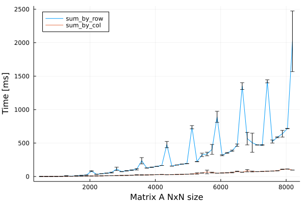
Now let’s explore how times are changing with matrix $A$ size ranging from 512x512 to 8192x8192.
Notebook with benchmarks is available at GitHub.
The summing mysteries
We can observe two interesting behaviors:
- Summing by columns first is constantly faster the summing by rows first.
- Summing by rows is not only slower, but also exhibits a peculiar irregularities.
The answer to the first question is as following.
The problem with traversing matrix by rows in julia is the matrix memory layout and how it interacts with processors cache memory.
When you access A[i, j], not only specific A[i, j] element is copied to processors cache, but a bigger chunk of continuous memory.
The computer predicts that if you’ve accessed A[i, j] element, you might want to access the next in the near future.
In a column-major memory layout as in julia, the next element is A[i + 1, j], so sum_by_col function is memory layout friendly (inner loop goes over i).
In the opposite in sum_by_row, when you use A[i, j] element, processor predicts that you may want to use A[i + 1, j] in the near future, while what you really need is A[i, j + 1], element that may be far away and require different part of memory copied into cache.
The second behavior however surprised me and I’m actively looking for the answer :)
How should I sum the matrix then?
Just use the provided sum function. :)
It takes care of the above effects and more.
However, when you have to traverse the whole matrix and conduct some more advanced calculations then it’s important to follow the memory layout if you want to be efficient.
Look forward to applicable examples in upcoming posts!