In the previous post I’ve presented the basics of stating mathematical optimization problems and JuMP framework in julia. Today let’s follow up with concrete examples! Please checkout the accompanying jupyter notebook even though you might not feel like a programmer. It’s very clear and shows how easy it is to obtain solutions!
Finding maximum garden area 🏡
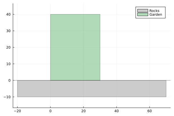
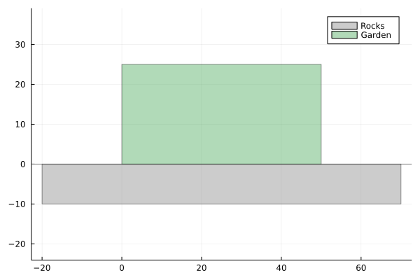
This one is the easiest. Imagine that you have to put a fence around your garden. You have 100m of fence. One side of your land is near rocks so you don’t have to waste fence on it. Your task is to find a way of putting the fence so it maximizes the are inside.
Problem can be easily translated into mathematical optimization problem:
$$ \begin{aligned} \max\quad & x y \newline \text{Subject to} \quad & x + 2y = 100.0 \newline \end{aligned} $$
Solution:
julia> value(x), value(y), objective_value(model)
(50.0, 25.0, 1250.0)
So $x = 50$, $y=25$ and the garden area equals $1250$. The result looked strange for me at first glance. It’s an obvious fact that square is the rectangular of maximum area from all rectangles with certain perimeter. Here however, one side is already covered by rocks so problem is a bit different and the optimal fence has shape of rectangular with sides 25 and 50. heh…
Size of square fitted in quadratic
Our next problem is finding the maximum area of the square that can fit inside parabola under some threshold $y_{max} = 10$. When you look first on this problem it seems complicated and not trivial. Let’s do a nice visualization first.
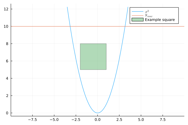
Our task is to maximize the green square area. To do so, our first observation should be that problem is symmetric with respect to line $x=0$. We can denote side of the square as $2a$. Instead of maximizing $(2a)^2$ we can just maximize $a$, this trick sometimes help solvers. It’s also pretty reasonable to say that top of our square will be aligned with line $y = y_{max}$. The bottom-right corner of square will have coordinates $(a, y_{max} - 2a)$. When square will be growing, it will grow until it hits a parabola so until it’s above $a^2$.
$$ \begin{aligned} \max\quad & a \newline \text{Subject to} \quad & 10 - 2 a \geq a^2 \newline \end{aligned} $$
julia> value(a), objective_value(model)
(2.316624802924551, 2.316624802924551)

julia> (2value(a))^2
21.467001910100855
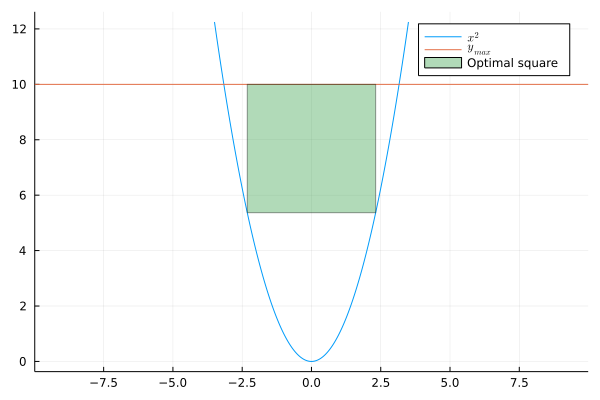
You might realise that this whole optimization was not necessary as the biggest square will have simply $10 - 2 a = a^2 $ and we can solve it for $a$. I highly encourage you to write it on paper and solve.
Size of rectangle fitted in quadratic
The above problem looked complicated at first but in the end we’ve discovered it can be easily solved via quadratic equation. Not let’s consider rectangle instead of a square. Suddenly the problems is (I think) out of bounds for high-school math and requires the basics of calculus to solve it by hand. Fortunately with our framework the problem is not that hard to write in JuMP. Let’s consider a rectangle of size $2a \times 2b$. We will be maximizing the area $(2a)\cdot (2b)$ with constraint $10 - 2 b \geq a^2$. This constraint will not be enough, we also have to make $a$ positive.
$$ \begin{aligned} \max\quad & (2a)\cdot(2b) \newline \text{Subject to} \quad & 10 - 2 b \geq a^2 \newline & a \geq 0 \end{aligned} $$
julia> value(a), value(b), objective_value(model)
(1.8257418674792618, 3.333333366323534, 24.343225140649853)
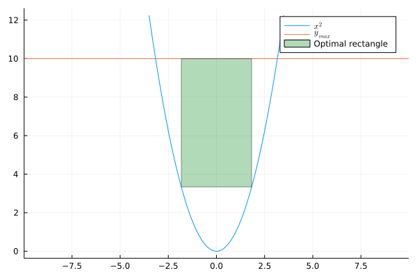
As with the previous problem, I highly encourage you to write this problem on paper and try to find the optimal $a$ and $b$ by hand, maybe with help of WolframAlpha.
Maximizing sales in a shop 🛒
John sells shirts. Right now he sells 16 shirts a day, £20 each. He observes that by decreasing price by £2 he is able to sell one shirt more. What is the optimal price of the shirt for John and what would be his profit then? Each shirt costs £5 to produce. It’s a typical Matura Exam question.
Let’s denote $n$ as number of shirts sold and $p$ as a single shirt price. For sure we know that our objective function is $n (p - 5)$ as we want to maximize John’s profit. Now we have to add some constraints.
The problem is tricky to write using only those two variables. Fortunately we can introduce new if we need! New variable $s$ will denote how many more shirts are sold. Now amount of sold shirts will be $n = 16 + s$ for price $p = 20 - 2s$.
If we had to do it on paper, we could eliminate $s$, find variable $n$ from constraints, and substitute it into objective function. We’re left with a simple quadratic depended only on $p$. That’s how we would solve it in high-school. With mathematical optimization framework we don’t have to this!
$$ \begin{aligned} \max\quad & n (p - 5) \newline \text{Subject to} \quad & n = 16 + s \newline & p = 20 - 2s \newline \end{aligned} $$
julia> value.([n, p, s]), objective_value(model)
([11.75, 28.5, -4.249999999999999], 276.125)
Here results require some interpretation as John might have trouble selling 11.75 shirts for total £276.125. The closest feasible solution is with $s = -4$, $n = 12$, $p=28$ with objective function £276. For John, surprisingly, he should raise the price to earn more.
Optimizing juice factory 🧃
The last example for today is the most exciting and involves numerous interesting tricks! Suppose that you are the Production Engineer at The Tasty Juice. You have 500kg apples and 300kg pears. You can create apple-pear juice by using 2kg of apples and 1kg pear. Current market prices are:
- 5€ for one kilogram of apples
- 7€ for one kilogram of pears
- 20€ for a liter of juice
How to maximize your profit?
It’s easy to write out our objective function, it’s just $5a + 7p + 20j$. Now we have to find some constraints. For sure we have to we can sell between 0 and 500kg of apples and between 0 and 300kg of pears.
But how to use some fruits for juice and sell the rest? We can introduce new variables! Apples used for juice $a_j$ and the same with pears $p_j$. Now constraints are $a + a_j \le 500$ and $p + p_j \le 300$.
It’s important to not write $0 \le a + a_j \le 500$, as it doesn’t restrict $a$ and $a_j$ to be positive, $a_j$ may be $5000$ and $a = -4990$ and still satisfy constraint.
So how to use fruits? We can force $p_j$ to be equal to $j$ and $2a_j = j$. The reasoning behind the second equation is that the number apples kilograms used should be twice as large as produced liters of juice.
Collecting everything, we can write: $$ \begin{aligned} \max\quad & 5 a + 7 p + 20 j \newline \text{Subject to} \quad & 2a_j - j = 0 \newline & p_j - j = 0 \newline & a \geq 0 \newline & a_j \geq 0 \newline & a + a_j \leq 500 \newline & p \geq 0 \newline & p_j \geq 0 \newline & p + p_j \leq 300 \newline \end{aligned} $$
Our solver solution is:
julia> round.(value.([a, aj, p, pj, j])), round(objective_value(model))
([-0.0, 500.0, 50.0, 250.0, 250.0], 5350.0)
This means that we should use all 500kg of apples and 250kg of pears to produce 250 liters of juice. We will sell it together with reminding 50kg of pears for 5350€ in total.
The summary of mathematical optimization
In this post I tried to show some simple problems solved by JuMP. If you have some ideas for modifications, download the notebook and play with it! Stay tuned for the next post, it will finally explain the math behind circles in circle!