In the post about fitting pizzas inside another pizza I’ve shown the following picture and promised a post about recreating it.
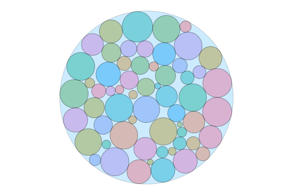
Pizzas packed in pizza
However, I would not like to assume that everyone is familiar with the optimization theory (you may graduate from Computer Science and still not know a lot) so I want to present an introduction here as high school math and quadratic equations are enough to understand those concepts.
Mathematical optimization for dummies
Mathematical optimization is usually just asking a question about finding values of some variables that minimize or maximize value of some function. We call this function the objective. For example:
$$ \min _x x^2 - 4x + 2. $$
With usage of high-school formula we can write:
$$ \min _x x^2 - 4x + 2 = \min _x \ (x - 2)^2, $$
and find $x_{\text{min}} = 2$.
Constrains in mathematical optimization
Often our optimization problem is constrained somehow. In the language of mathematical optimization we say that some variable is subjected to. We can introduce two types of constrains:
- Inequality constraint e.g. $x \le 4$
- Equality constraint e.g. $y = x - 5$
For example:
$$ \begin{aligned} \min\quad & x^2 + 5 \newline \text{Subject to} \quad & 4 \le x \le 10 \newline \end{aligned} $$
and here solution is $x_{min} = 4$ and objective function is $4^2 + 5 = 21$. Note that the interval is closed. It is super rare for optimization problems to have open boundaries. Try to think what it would mean.
Let’s consider:
$$ \begin{aligned} \max\quad & 4y \newline \text{Subject to} \quad & x \le 3 \newline & x = 2y + 2 \newline \end{aligned} $$
It may not be as obvious at first but $x_{max} = 3$, $y_{max} = 0.5$ with objective equal to $2$. What is interesting here is that we maximize over variables $x$ and $y$, while $x$ is not explicitly present in our objective function. Of course we may rewrite the problem by substituting $y$ by $x$. $$ 2y = x - 2 \newline y = (x - 2) / 2 \newline $$
$$ 4y = 2(x-2) = 2x - 4 $$
$$ \begin{aligned} \max\quad & 2x - 4 \newline \text{Subject to} \quad & x \le 3 \newline & y = (x - 2) / 2 \newline \end{aligned} $$
Problem written like this is much easier to solve by hand, and we eliminated one variable.
Solving optimization problems using julia
Let’s try to phrase above problems using julia.
We will be using JuMP package as it has a convenient interface.
The code is so self-explaining that I leave it as is.
At GitHub you will find a jupyter notebook with this code.
This is the first simple quadratic problem:
model = Model(Ipopt.Optimizer)

@variable(model, x)

@objective(model, Min, x^2 + 5 )
@constraint(model, 4 <= x <= 10)

optimize!(model)
To get the value of variable $x$ and objective function:
julia> value(x), objective_value(model)
(3.0000000297721905, 35.00000032749409)
And the second problem with two variables:
model = Model(Ipopt.Optimizer)

@variable(model, x)
@variable(model, y)

@objective(model, Max, 4y)
@constraint(model, x <= 3)
@constraint(model, x == 2y + 2)

optimize!(model)
julia> value(x), value(y), objective_value(model)
(3.000000028747048, 0.500000014373524, 2.000000057494096)
The two paths in mathematical optimization
What I haven’t said yet is that there are two main paths in optimization field:
- Writing problems in framework presented above.
- Writing solvers for those problems.
Those problems are surprisingly separable. You may have strong skills in formulating optimization problems and doesn’t have any clue about low-level processor optimization. Similarly you may love to find all the weird SIMD optimization and be careful about memory patters and doesn’t really care what are you calculating.
Why this post was interesting?
While problems described above may not be so fascinating, they serve as good examples how to write problems in mathematical optimization framework.
Stay tuned for the next mathematical optimization post in which we will solve some imaginary real-life problems using JuMP!!!