In a recent post, I presented how memory layout may influence a matrix summing speed. It’s interesting to see that there are plenty of pitfalls we might fall into when writing sum function and memory layout is not the only one. Please first read the previous post on summing if you haven’t already.
Without thinking why, let’s take a look at those two functions:
function sum1(A)
    s = zero(eltype(A))
    n, m = size(A)
    @assert n == m
    sv = zeros(n)
    for i in 1:n
        for j in 1:n
            sv[j] += A[i, j]
        end
    end
    for i in 1:n
        s += sv[i]
    end
    return s
end
function sum2(A)
    s = zero(eltype(A))
    n, m = size(A)
    @assert n == m
    sv = zeros(n)
    for i in 1:n
        for j in 1:n
            sv[i] += A[i, j]
        end
    end
    for i in 1:n
        s += sv[i]
    end
    return s
end
They are very similar to the efficient function from the previous post, but now we’re not summing into a single variable. Instead, we first calculate a sum for each row/column and then sum the intermediate row/column result. As we will soon see, adding this additional vector may change something.
Benchmarking different summing approaches
There are 4 ways of summing I’d like to compare:
- Calculate sum of each row of $A$ into vector
svand then calculate sum ofsv–for_row. - Calculate sum of each column of $A$ into vector
svand then calculate sum ofsv–for_col. - Calculate sum of the whole $A$ using one variable only (as in a previous post, IMHO the most intuitive way of summing a matrix) –
simple_sum. - Calculate using built-in function
sum–Base.sum.
Each function will be benchmarked on a random matrix $A$ which size ranges from 512 to 8192.
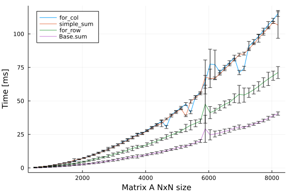
Findings:
- Creating intermediate vector for sums of each row made function run 30-40% faster when compared to the simple summing function without additional vector.
- Creating intermediate vector for sums of each columns is slightly slower then our previous summing method.
- As we might expect, the built-in
Base.sumfunction is even faster.
Why creating additional array made function run faster?
Finding #1
So this is one of these problems where at first results are strange, but a moment later they’re obvious. The key factor is a low-level parallelization that the processor is able to perform when calculating sums for rows.
First, observe that in general, the summing operation is not parallelizable. If you want to calculate sum of array $[1, 2, 3, 4]$ by visiting each element in turn, you have to calculate $0 + 1$, $1 + 2$, then $3 + 3$ and finally $6 + 4$. You could at one time calculate $1 + 2$ and $3 + 4$, and then do $3 + 7$ but it would require jumping over the array.
Not let’s remind that julia has F-style memory layout with a matrix being stored as a sequence of columns. This means (as discussed in a previous post) that to iterate along the memory, we have to iterate with the outer loop over columns and the inner over rows.
Imagine that you have to sum elements of the following matrix $A$:
$$ A = \begin{pmatrix} 1 & 2 & 3 \\ 4 & 5 & 6 \\ 7 & 8 & 9 \end{pmatrix} $$
by traversing it’s elements in the above order i.e. traversing a vector $A_F = [1,4,7,2,5,8,3,6,9]$.
If we would like to calculate sum of $1+4+7$ first into sv[1] you throttle on access to sv[1] element.
Computer have to wait for the result of $1+4$ until it is able to add $7$.
Please note that after we’re done with column 1, sv[1] is not used any more except for the final sv summing.
Calculating sum of rows is a different story however!
Processor can simultaneously add $1$ to sv[1], $4$ to sv[2] and $7$ to sv[3].
Only then it has to wait until $1$ is added to sv[1] to proceed with the second column. And the third.
Finally there is a place for optimization.
The only throttling operation is calculating the sum of sv vector in the end.
Finding #2
This one is rather obvious, small overhead has been added with this new vector without any place for optimization.
Finding #3
I was curious how sum is performed in julia and I was surprised by the level of it’s both beauty and complexity.
The beauty lies in the form that sum(A) is more or less defined as reduce(+, A), which is mapreduce(identity, +, A).
This makes functions sum and prod(A) = reduce(*, A) function (probably also a few more) share almost the whole code base (prod is product, i.e. prod([2, 3, 4]) == 24).
Complexity lies in a way mapreduce function is written.
This implementation takes advantage of low-level optimizations.
How should I write my code based on these experiments
In this post, we discovered another thing to keep in mind when writing high-performance code. First, try to use built-in methods when possible. Second, try to design the function in a way that there is no way for throttling on access to a single variable. Thinking in this way also allows performing some higher-level optimization when necessary.